Digging to the roots - the theory behind hydraulic turbines and pumps
13 August 2008Hungarian mathematician and mechanical engineer, Dr Arpad A Fay had his first international paper published in IWP&DC in April 1970. In August 2008, Dr Fay is 75 years old. Here he recounts his vast experience of researching the theory behind hydraulic turbines and pumps
Arpad Fay joined the hydro machinery laboratory of GANZ, the only hydraulic turbine manufacturer in Hungary, as a research assistant in 1957. His first job in the laboratory was the cavitation testing of Kaplan models. After three years of almost continuous testing he proposed to redesign the test rig. In checking the design his managers expressed some doubts but Fay defended the design saying: ‘If Newton’s laws are valid, then this will work properly.’
This proved to be correct as Fay’s test rig was used for more than 40 years. He retained the same philosophy till his retirement from GANZ in 1998. ‘Dig to the roots if time permits’ he told his students in the University of Miskolc, where he was a part-time lecturer from 1989. His favorite research subject was the theory of hydraulic turbines and pumps. A collection of his results is presented below.
Torque equation of runners
In the laboratory Fay measured velocity distributions upstream and downstream of Kaplan runners with three-hole cylindrical probes (Figure 1). Surprisingly, the difference in the incoming and outgoing moments of momentums Timpuls, Equation (1), did not agree with the shaft torque Tshaft (transmitted through Ashaft, Figure 1).
This seemed to be a hard blow to the theory of turbine design since it had been based on Euler’s turbine equation derived from the equality of these torques.
To find a solution to this basic question Fay estimated various errors, made special tests, returned to the basic laws of mechanics, and following Csanady [1] applied the moment of momentum theorem to the mass enclosed by the control surface shown by the dotted line in Figure 1.
Considering the torques on the control surface Ashaft+Ain+Acasing+Aout+Ahub (Figure 1) and neglecting very small terms, Equation (2) was derived. This states that Timpuls is almost balanced by Tshaft but two correction terms: Tcasing, the friction torque exerted on the casing, and Tturbulence, Equation (3), the torque due to Reynolds stresses on inlet and outlet parts of the control surface. Thus, Equation (2) explained the difference of the main torques obtained from the experiments.


Equation (2) plays the same central role in the theory of turbo machines as before the Euler equation [1]. Fay derived simple estimates for the correction terms [2]. To estimate the Reynolds stresses downstream from the runner, simple wake flows were assumed for the blades in the relative velocity field. In the absolute velocities this resulted in realistic values for the Reynolds stresses. This little trick enabled the use of Equation (2) in the design during the 1960s. Today, Equation (2) is consistent with modern 3D turbulent flow computations since the computed Reynolds stresses may be substituted.
Scale effects
Professor SP Hutton, the head of the Mechanical Engineering Department at the University of Southampton in the UK, invited Fay to Southampton in 1971 to write a study on scale effects for the international-electrotechnical-commission’s (iec) standardisation. After completing the study he became a member of Working Group 18 (scale effects) of IEC/TC4 (hydraulic turbines) for 25 years. He also kept in contact with Professor J Osterwalder’s Darmstadt circle at the International Association of Hydraulic Engineering and Research (iahr WG5), which was also involved in scale effects. This enabled him to compare the results of three important scale effect working groups (Table 1) [3].
The scale effect was calculated by the standard formula:

where ?hM is the hydraulic efficiency of the model (directly measurable with the model), ?hP is the hydraulic efficiency of the hydraulically smooth prototype, Re is the Reynolds number (as defined in IEC 60193), M and P stands for model and prototype respectively, a = 0.1e (as suggested by Osterwalder), and V is the loss distribution coefficient (Figure 2).
The IEC collected V values from various firms but the statistics showed a large scatter due certainly to the large uncertainty in the field tests. Therefore a single average was calculated (Figure 2), which is near to the rounded value 0.7, recommended for Francis turbines in IEC 60193. The curve published by Osterwalder [5] is based on the work of high accuracy leading laboratories. His values are somewhat larger than the average outcome of the Japanese computations [6]. The difference is not too large, and so for present use Fay suggested [3] an average curve (Figure 2).
The standard scale formula, Equation (4), is based on the Reynolds numbers, and therefore it is valid theoretically only if both model and prototype are hydraulically smooth. This condition can be assured for models with suitable surface finish but for prototypes this may not be economical. This problem was studied recently by Krishnamachar and Fay [7].
In these calculations the roughness is represented by Ra, the root mean square of the protrusions in microns (which is the surface roughness value given in manufacturing drawings). Table 2 includes five sets of assumed roughness values for a Francis turbine of medium specific speed ?q = 50, together with the calculated drop in the prototype efficiency.
The last column gives an idea about the magnitude of the roughness effect. If the specific speed of the prototype largely departs from ?q = 50, then the calculation can easily be repeated [3]. In practice, one may accept an efficiency allowance DhP for the prototype roughness, and using such a table an allowable prototype roughness can be determined. In this way the gain of using a suitable surface finish technology may also be evaluated. In our age when both models and prototypes are produced with numerically controlled machines the geometric similarity of model and prototype runners is almost perfect. Since more exact runners imply more regular scale effects; the trust in the scale formulae is growing all over the world.
Cavitation noise
In the Technical University of Budapest cavitation noise and damage tests were made in a cavitation tunnel by Professor JJ Varga and Dr G Sebestyén [8,9]. The practical implementation of the results to model turbines and pumps was arranged by Dr Fay.
It was well known that cavitation has the most marked effect in the noise spectra around 100kHz. The commercially available Bruel & Kjaer instruments, however, covered only the sonic range up to 20kHz. Nevertheless, Varga and Sebestyén [8,9,10] found that these instruments may still provide useful information on cavitation.
The effects of cavitation are typical even in the range of 10-20kHz, while other noises (motor, pump, other flow-born, environmental) are usually negligible in this range. The sound pressure level np was measured by a condenser microphone, and the vibration level ng by an accelerometer. Making the cavitation test in the tunnel with decreasing s, including sound or vibration level measurement at constant frequency in the above range, the ?p(s) or ?g(s) curves showed first an increasing section (developing cavitation) and after reaching a maximum, the level decreased (exhausting cavitation).
The ?p(s) and ?g(s) curves resulted always in the same developing and exhausting s ranges. The placement of the sensors did not affect these ranges either. Cavitation damage tests were also made with lead plates placed to the wall of the cavitation tunnel. These proved that maximum damage rate was obtained at the same s where maximum noise or vibration was observed. Thus, the s value of the most dangerous condition could be determined from the ?p(s) or ?g(s) curve [8,9].
The above statements are valid for hydraulic turbines and pumps as well [10], except that the ?p(s) or ?g(s) curves always showed two peaks for a Francis model, as in Figure 3. Comparing the ?p(s) curve of Figure 3, the hump above s = 0.25 may be associated with the development of the cavitation rope in the draft tube, while the hump below s = 0.25 describes runner cavitation. In general, a single hump on the ?p(s) curve is characteristic to one type of cavitation developing in one area, and two humps indicate two types of cavitation.
Such noise tests are not suitable to predict cavitation damage for the prototype but at least some orientation may be obtained for the s values about the most damaging operating conditions. This is useful in the case of new projects to select a suitable runner level, or in the case of existing turbines to change the operating condition to have less damage.
Karman vortex rows
Vortex rows downstream in cylinders have attracted the most research in fluid mechanics. Von Karman developed a stability theory which explains why the vortex row remains stable for the downstream generating body. However, he did not deal with the near-body mechanism, ie how can vortices of essential circulation appear in practically inviscid fluids. This question is also important for hydraulic turbines since in downstream vanes or blades similar vortex rows are formed when it operates near the best efficiency point.
Evaluating the high speed films of cavitating vortex formations by Varga and Sebetyén [9], Fay developed a simple theory for the vortex formation [11]. A few shots are sketched from the film in Figure 4. The top sketch shows a small jet initiation in the main cavity attached to the wedge model. Later the jet crosses the cavity, and on reaching the opposite side a vortex cavity of essential circulation is separated from the main cavity. Then, after a few moments a jet forms on the other side of the main cavity, and so alternate jet formations generate the von Karman vortex row. Fay computed jet formations in wake cavities [12], and there is also experimental evidence that in non cavitating flows the vortex formation mechanism is similar [11].
Rotating stall in Francis runners
Computations are more difficult in flows with boundary layer separations than those without it. Fay studied flow separations in 2D flows [13], and also in hydraulic turbines [14]. It is logical to assume flow separations in runners when the blades operate with a large attack angle. Krishnamachar, Fay and Rangnekar studied this problem [15]. They assumed rotating stall in Francis runners as in pumps and compressors. This may explain the occurrence of spiraling flows in draft tubes.
There is however another theory for the spiraling flows [16,17] based on the movement of the fluid mass in the draft tube. Further research is needed to sort out the connection between the two theories. This is important since spiraling flows are closely related to the power fluctuations of Francis machines. The role of rotating stall in Francis runners is the present research subject of Dr Fay who welcomes contributions from others.
Dr Arpad Fay can be contacted by email: Arpad.fay@t-online.hu
TablesTable 1 Table 2