Monitoring behaviour
17 November 2005Isabelle Penot, Bruno Daumas, and Jean-Paul Fabre report the methods used by EDF to monitor the behaviour of dams
The main aim of monitoring major civil engineering structures is to provide an early warning system for any significant change in behaviour. The monitoring principle is thus a simple one: detecting any sign of a change of behaviour as early as possible, by highlighting phenomena that are evolving over time.
In order to make a judgment on the behaviour of the structure, high quality measurements are needed. This data then needs to be correctly used – that is, all means available need to be used to draw out the maximum useful information.
The simplest approach is to transfer points to represent these phenomena onto a graph displaying time and the amplitude of the phenomena measured, then compare the position of all new points with the historical data cluster.
This type of display can prove extremely useful in monitoring certain processes, particularly when very few reversible phenomena are involved.
However, on this type of graph, data can tend to be widely scattered due to external reversible influences that act on the condition of the structure any moment in time (level of water in the reservoir in front of the dam and thermal conditions). A graph of raw data is not easy to analyse and conclusions are difficult to draw. As the data cluster is often highly scattered, gradual trends or small anomalies can be very difficult to identify, particularly when they are major external influences.
edf is therefore looking to identify statistical analysis models that can separate the various explanatory factors and extract useful data that is not influenced by these factors. The aim is to ensure that operational monitoring of the structures is based on measurements that have been ‘corrected’. Such a process facilitates comparison between measurements and the identification of any anomalies and, in particular, irreversible changes. Moreover, it is important that so-called reversible effects are well understood, providing invaluable information on the behaviour of the structure, so that the phenomenon observed can be fully understood.
Research method
The following method was used to identify statistical analysis models for measurements used by EDF in monitoring dams:
• Identifying external influences at determining structure behaviour, eg. reservoir water level, acting on the dam as hydrostatic force resulting from water pressure.
• Determining the variables that can explain or represent the influences mentioned above, eg. relative trough z, representing the reservoir water level, determined by the following relation

where RN is the normal reservoir level, Rvide the empty reservoir and h the actual water level in the reservoir.
• Identifying an algebraic function for the ‘explanatory’ variable. The aim is to find a function whose shape translates the influence of the phenomenon as accurately as possible, eg. the hydrostatic effect is modelled by a polynomial function of the relative trough z, to the 4th degree at the most.
• Adjusting the model to a calibration frequency selected across all the measurements already taken (least squares method).
• Critiquing the adjusted model, in particular by analysing the quality of the explanation given by the coefficient of determination R2, and analysing the reversible effects obtained.
• Calculating the corrected measurements (raw data adjusted to take reversible effects into account).
Thermal HST Model
The so-called HST method (Hydrostatique Saisonnier Temps – hydrostatics, seasonal factors, time) was developed by EDF for monitoring dams (Wilm & Beaujoint, 1967). This statistical analysis method is based on a mean seasonal thermal reference value for the phenomena observed on the dams, and it enables regular variations to be identified according to the reservoir level and the date in the year.
This easy-to-use method has proved to be an effective and powerful interpretative resource in analysing the behaviour of structures. However, the HST model has an inherent limitation in that it assumes that the thermal effects can be modelled using a seasonal distribution with a one-year cycle. The HST based data corrections are not particularly relevant during periods when thermal conditions are unusual for the season, especially so for thinner dams.
Our aim was to improve the HST method on the basis of the above observations. We attempted to fine-tune the model, particularly at its weakest point, the modelling of the thermal effect, by using real temperature data, whilst retaining the hydrostatic, seasonal and irreversible functions in the new model.
External influences
Two types of phenomena influence the deformation of concrete structures. Some cause reversible movements, such as the reservoir water level, when water in the reservoir produces hydrostatic pressure on the structure, and temperature distribution within the structure, when variation in the temperature range in the structure leads to deformation.
Other influences lead to irreversible movements, such as creep, fatigue and swelling phenomena, which act over all or part of the structure's life.
Selection of variables
It is assumed that the raw measurements taken on concrete dams represent the sum of three main states:
• An irreversible state, which represents an evolving phenomena over time t, which may tend to be counteracted (adaptation or consolidation) or accelerated (damage).
• A reversible state that corresponds to the effect of hydrostatic pressure, as represented by the relative trough z.
• A reversible state linked to the temperature conditions Q of the structure. (According to the HST model, it is assumed that each year, at the same date, the structural deformation due to the thermal conditions is the same, depending solely on the season S, which is represented by a curve, on which the 0° angle is 1st January and 360° the 31st December).
We therefore find that for an observed value Xi described in the phenomenon, three functions f1(t), f2(z) and f3(?) exist, such that:
Xi = f1 (t1) + f2 (zi) + f3 (Ti)+ ei
where t, z and T represent the specific current values for the variables as taken on the day of measurement.
The term e represents all experimental errors and inaccuracy inherent in the model (the effects of all other influences which are assumed to be secondary and are left out for the purposes of simplification).
Algebraic expression of the model
f1(t) distribution
This distribution comprises up to five different terms: Evolution over time, represented by terms directly linked to the time t: t, t2, t3 and t4, and a counteracted evolution, represented by a negative exponential function of the time e-t/t (t set by the user).
f2(z) distribution
The hydrostatic distribution is given by a polynomial function of the relative trough Z (to the 4th degree at the most).
f3(Q) distribution
It is in this respect that the upgraded HST Thermal method is considered innovative.
Influence of the air temperature
After many years using the HST method, it has been established that approximating the thermal effect to an average seasonal distribution can, overall, give relevant corrections in the vast majority cases.
Nevertheless, due to its very construction, the HST model cannot take real temperature variations into account. Hence, for phenomena which are sensitive to such variations, the residual scatter of measurements corrected using the model may remain high and at the time the model does not give relevant results (during periods that are hotter or colder than usual, such as the heat wave in Europe in summer 2003, for instance).
In the HST Thermal model, it is assumed that the major factor in thermally-induced movements is the air temperature.
Now, for each day, j, the daily air temperature Q (j) can be broken down as the sum of the normally expected temperature for that day N (j) and the difference between the actual temperature and this normal temperature ? T (j) as follows:
T(j)=N(j)+?T(j)
(where N(j) is a seasonal trigonometric function with a 1-year cycle).
The air temperature variations (main factor) generate a range of temperatures within the body of the structure, which in turn leads to thermally-induced displacement (effect) transmitted via the structure's thermal inertia (leading to a delay and attenuation in the input signal).
Table 1 gives a schematic description of the principle use to model the thermal effect in the H.S.T. Thermal method.
The following hypotheses can thus be used to improve the representative distribution of the thermal effect:
• Continuing to use a seasonal function in expressing this distribution (to represent an average year of thermal variations): the seasonal function shows the delayed reaction of the structure to the annual periodical variations in temperature (gradual evolution).
• Completing and correcting this seasonal function is by taking into the account the difference between the observed daily temperatures and the normal value for the time of year. This corrective function is used to take into account the structure's delayed reaction to rapid daily variations in air temperature.
Thermal correction function
The thermal correction function is determined as shown in Table 2.
The variable of delayed difference
representing the differences between the observed temperature and ‘normal’ temperature is calculated as follows:

The variable DQR is thus configured using a time value T0, which is dependent on the geometrical and thermal properties of the structure.
This variation distribution comes very close to that of the average temperature of a wall with finite thickness subject to t ?T external temperature variations (this is the first term in its Fourier series).
Thermal effect
The full distribution for the thermal effect in the Thermal H.S.T. model is thus the sum of:
• A seasonal effect (identical to the H.S.T. model), with the following form: b10 cos(S) + b11 sin(S) + b12 sin(2S) + b13 cos(2S)
A thermal correction function, specific to the HST Thermal model, proportional to the difference in the daily temperature as compared to the seasonal ‘normal value’ delayed in time (this function includes a "thermal sensitivity" coefficient, K), and is modelled in the following form: K ? TR [2].
Algebraic expression of the model
In full, this distribution is expressed as follows:
Xi = b0 + b1t + b2ti2 + b3ti3 + b4ti4 + b5e-ti/t
+b6Zi + b7Zi2 + b8Zi3 + b9Zi4
+b10 cos(Si) + b11 sin(Si) + b12 sin2(Si) + b13 sin(Si) + K?TR[T0] (ti) + ei
where b0 is a constant that takes into account the arbitrary origin of the phenomena. The parameters are calibrated using the least squares method.
Interpretation of specific parameters K and T0 for an arch-dam
Parameter K
This is an indicator of the thermal sensitivity of the structure in question, in terms of behaviour under strain. It is an expression of the variation in the value of the phenomenon measured over a prolonged 1°C increase in air temperature.
The main factors determining the sensitivity are the geometry of the structure and the properties of the concrete used. Indeed, using a model to describe displacement in the crest of the arch caused by heating, under certain assumptions (free arch, circular, both ends half-embedded, heating leading to deformations (50 %) and stresses (50 %), it can be demonstrated that radial displacement at the crown cantilever due to the thermal effect can be expressed as:

where R is the upstream radius at the dam crest, ?the expansion coefficient of the concrete and ?T the average thermal heating of the concrete.
In this case, the thermal sensitivity coefficient K links the effect (thermal displacement dR) to the source (thermal heating ?T), with the relation: dR = K.?T.
The theoretical approach thus enables us to define the sensitivity coefficient K in terms of: a thermal property of the concrete: expansion coefficient ?; a geometrical property of the structure: radius R.
Hence K can be expressed as follows:

Note: Given a mean value for ? of 10-5/°C, the above formula can give an expected order of magnitude for coefficient K at the crown cantilever of a structure of radius R:

i.e. for a structure with a 100 metre radius,

Parameter T0
T0 is an indicator of the structure's thermal inertia.
The thermal inertia of a dam is usually characterised not by T0 but by another time, given as T90. T90 represents the time taken for the structure to reach 90 % of the final phenomenon value. With the selected distribution, T90 = ln(10).T0 ˜ -0.75 mm/°C.
It can be demonstrated that, in particular, this time T90 depends on the structure's geometry and the properties of the concrete used. Indeed, if the effect of upstream water is left to one side, the equation for heat in a finite medium of thickness e and diffusivity a can be solved such that T90 is expressed as this approximation:

The theoretical approach thus enables us to determine the time T90 which characterises the structure's inertia in terms of: a thermal property of the concrete: diffusivity a; a geometrical property of the structure: equivalent thickness e (for arch dams, the thickness at dam crest).
Hence T90 can be expressed as follows:

(where e is the thickness expressed in meters and a, the diffusivity expressed in m2/j).
Note: Given a medium value for a of 9.36x10⁻²m2/j, the above formula can give an expected order of magnitude for time T90 at the crown cantilever of a structure whose thickness at the dam crest is e:

i.e. for a structure whose thickness at the dam crest is 4m

Operation examples of the HST Thermal modelStructure A: displacement measurements using pendulum
The geometrical properties of the structure are: upstream radius at dam crest, 65m and thickness at dam crest is 2.5m.
With these properties, the expected values for displacement of the dam’s crown and crest using the HST Thermal model should be close to:
T90 = 16 days,
K = -0.5 mm/°C.
221 measurements are available for the period analysed (1995-2003). For the data series analysed, the HST Thermal model gives a 58 % reduction in scattering (in comparison with corrections made using HST).
During the unusual climatic conditions in the heat wave of summer of 2003, it can be seen that the HST model's corrections were wrong (see figure 2), showing an unexplained upstream displacement of the order of 5mm. It can also be shown (see figure 4) that during this period, the HST Thermal module can give a suitable expectation for a 4 to 5mm displacement upstream that could not be analysed using HST. This explains the way the heat wave was well corrected on the graph of data corrected using HST Thermal (see figure 3).
The parameters of the model (T90 = 20 days, K = -0.65 mm/°C) are, moreover, consistent with the geometrical properties of the structure.
Structure B: displacement measurements by planimetry
The geometrical properties of the structure are: upstream radius at dam crest is 62.5m and thickness at dam crest is 3.5m.
With these properties, the expected values for displacement of the dam’s crown and crest using the HST Thermal model should be close to:
T90 = 31 days,
K = -0.45 mm/°C.
89 measurements are available for the period analysed (1995-2003).
For the data series analysed, the HST Thermal model gives a 36% reduction in scattering.
The parameters of the model (T90 = 27 days, K = -0.47mm/°C) are, moreover, consistent with the geometrical properties of the structure (see 0).
Advances provided by the HST Thermal model
The HST Thermal method has the following advantages:
• Extremely effective corrections: in the vast majority of cases, the displacements at the crest of thin arches are very well explained,.
• Accurate modelling of the thermal effect, taking into account the effect of the temperature, cyclical and gradual variations as well as rapid variations.
The contribution of the HST Thermal model over and above the ‘traditional’ HST method can be quantified as follows:
• During an usual meteorological episode, the explanation put forward can be assessed in terms of thermal correction, in addition to the seasonal translation function,
• On a ‘macro’ level, throughout the period analysed, HST Thermal reduces the scattering of corrected data as compared to a traditional HST analysis.
• This reduced scatter reduces the proportion of the scatter that cannot be explained by the model within the chronological series of raw measurement data. That is to say, the model has an increased explanatory quality.
In the context of operational monitoring of the structures, reduced scatter means anomalies can be better detected (by eliminating the reversible effect) and the structure's behaviour can be better diagnosed (by reducing residual scatter). This improvement can be retrospectively applied (drafting monitoring reports), or in real-time (studying current data).
Across EDF's 48 arch dams in France, applying the HST Thermal model will contribute significant added value over HST. The figures show that for the sample analysed, the reduction in scatter of the corrected data between HST analysis and HST Thermal analysis: Is 40 % on average; Can be as high as 65 %; Is over 50 % for one quarter of all structures.
This method is already used by EDF, bringing significant added value in the diagnostics of structure behaviour and increasing the quality of analysis.
Author Info:
The authors are Isabelle Penot, Bruno Daumas and Jean-Paul Fabre of EDF. For further information, email: isabelle.penot@edf.fr
TablesTable 1 Table 2